
Over the last few years, I’ve noticed a marked increase in the number of companies that are worried about their analytics data becoming contaminated with non-human traffic – and with good reason. According to a fairly recent report from Imperva, websites that have more than 100k human visitors everyday should expect nearly one third of their traffic to be caused by bots – a startling figure! This is a major problem for analytics and testing when you realize that most marketing campaigns or product testing successes are based on the conversions per visitor. If one third of the “visitors” to your marketing campaign or A/B test are not human at all, it becomes difficult to trust the results of any optimization, analytics, or attribution tool.
So, how can you determine the impact bots have on your Adobe Analytics data? Well it’s complicated, and in this post I’m going to illustrate the different types of bots out there and the types that can impact your analytics data. I’ll also give you some strategies for filtering them out so you can avoid making bad marketing or product decisions based on bad, bot-tainted data.
To start, it’s important to understand the different types of bots that are visiting your site:
- Basic Dumb Bots: These types of bots are based on very simple http requests to your site to download its HTML content. Dumb bots don’t execute JavaScript, so they never show up in your Analytics data. They may represent a significant portion of the traffic to your site, but there’s really nothing to worry about here with respect to analytics data.
- Good Bots: These bots are much smarter and will typically execute any JavaScript on your site (including your analytics tags). Examples of good bots include site monitoring bots, search engines, tag auditing tools, and feed fetchers (bots that fetch your site content typically for displaying in a mobile app – think Flipboard or Apple News). Good bots are fairly easy to filter out from Adobe Analytics because they typically self-identify via their user agent string. The easiest way to filter these types of bots from Adobe Analytics is to enable automatic bot filtering which you can read how to setup here.
- Bad Bots: This is where things get really messy. Bad bots are bots that are doing things on your site that you probably don’t want, and are typically sophisticated and hard to detect because they try to avoid detection. In fact, there is no general industry consensus that I’ve heard about around exactly how common these bots are, but most agree they have become more common than good bots. The most common types of bad bots I see come from competitors’ price scraping tools, impersonators used to commit ad fraud (oftentimes this is malware in people’s browsers inflating clicks to a site’s advertising), spam bots used to inject unwanted links into site forums and comments, and hacker tools that are looking for security weaknesses in your site.
Anecdotally, I tend to hear a lot more about bots from companies that compete on price. Travel and hospitality are usually the most heavily hit, but I’ve heard of some retailers that are also especially hard hit – to the point where they believe over 30% of the unique visitors in their data are actually bots!
So, how do you quantify the impact of bots on your data? There is an entire industry out there dedicated to answering this question (my favorites are ShieldSquare, PerimeterX, and WhiteOps), but if a bot detection vendor isn’t the path for you, using Data Feeds with R can still really help. If you haven’t read my post on setting up sparklyr, the R interface for Apache Spark, you’ll want to check that out first because we’ll be relying heavily on sparklyr for this post. But before we start coding any R, you’re going to need to setup a Data Feed with a few key variables: post_visid_high, post_visid_low, user_agent, hit_time_gmt, ip, browser, and os.
Next, we’ll load the data into Spark and prep the data with the proper lookup tables that come included with the Data Feed:
library(dplyr)
library(sparklyr)

# Read Data Feed Files Into Spark
sc = spark_connect(master="local", version="2.1.0")
data_feed_local = spark_read_csv(
  sc=sc,
  name="data_feed",
  path="data/report_suite/01-report_suite_2017-*.tsv",
  header=FALSE,
  delimiter="\t"
)

# Read Column Headers File & View For Reference
col_names = read.csv(
  file="data/report_suite/...lookup_data/column_headers.tsv",
  header=FALSE,
  sep="\t"
)
View(t(col_names))

# Read Lookup Files From Data Feed
browsers_local = spark_read_csv(
  sc=sc,
  name="browser_lookup",
  path="data/report_suite/...lookup_data/browser.tsv",
  header=FALSE,
  delimiter="\t"
)
os_local = spark_read_csv(
  sc=sc,
  name="os_lookup",
  path="data/report_suite/...lookup_data/operating_systems.tsv",
  header=FALSE,
  delimiter="\t"
)

# Assign Headers to Browser & OS Lookup
browsers_tbl = browsers_local %>%
  select(
    browser = V1,
    browser_friendly_name = V2
  )

os_tbl = os_local %>%
  select(
    os = V1,
    os_friendly_name = V2
  )
With the data loaded, we can prep it and give the columns a more friendly naming scheme, and apply the browser and os lookups using a left join:
# Create a sparklyr data frame for analysis
data_feed_tbl = data_feed_local %>%
  mutate(
    visitor_id = paste0(V1,"_", V2),
    browser = V14,
    os = V21
  ) %>%
  left_join(browsers_tbl, by="browser") %>%
  left_join(os_tbl, by="os") %>%
  select(
    visitor_id,
    timestamp = V4,
    browser_friendly_name,
    user_agent = V3,
    ip_address = V5,
    os_friendly_name
  )
Now we’re ready to have some fun! Before the next bit of R code, I should probably explain a couple things about bots. Bots very frequently have a few characteristics that humans don’t. Bots will often originate from AWS, Google, or some other cloud provider, they often don’t accept cookies (making each hit its own unique visitor), they are very frequently coming from a Linux or unknown operating system, and will frequently have a spoofed user agent string that results in an outdated or unknown browser version. That stuff is pretty easy to identify (and quite effective all by itself). The trickier bots will use ip addresses and user agents that aren’t easily blocked, which makes things more difficult. To pinpoint those trickier bots, we’re going to use a statistical technique known as linear regression. Allow me to explain.
When a bot sends in a hit every 5 mins or every 15 mins or every hour, those timestamps are extremely predicable and leave a statistical trace in the data. When a human sends in hits, the hit interval is very unpredictable because it’s based on a human actually clicking around on a website. A good statistical test can identify how predictable the hit interval is – this is where linear regression can help. One way to think of linear regression is that it is a statistical test that can measure how well a linear model fits (or how well it predicts) a set of data. Linear regressions applied to extremely predictable signals have a coefficient of determination (or r squared value) very close to 1, while signals that are not as predictable (meaning the regression doesn’t fit the data as well) will be significantly less than 1.
To get all these data points in the format I need, I’m going to use the following R code:
ipua_rollup = data_feed_tbl %>%
  # Notice I group by ip, ua and os and not by visitor ID
  # since every bot hit can be a new visitor
  group_by(ip_address, user_agent, os_friendly_name) %>%
  mutate(
    # Here I'm normalizing the timestamp so the
    # numbers aren't so large
    y = timestamp - min(timestamp),

    # Here I'm setting up the independent variable
    # for the regression. I'm going to use a very
    # predictable sequence (the row number) to see
    # how well it can predict the timestamp.
    x = row_number(y) - min(row_number(y))
  ) %>%
  arrange(y) %>%
  summarize(
    # Here's the crazy R squared formula for
    # linear regression you learned in your
    # college statistics class...
    r_squared = ((n()*sum(x*y)-sum(x)*sum(y))/
      sqrt((n()*sum(x^2)-sum(x)^2)*
      (n()*sum(y^2)-sum(y)^2)))^2,

    # Here are all the other data points I need
    hit_count = n(),
    visitor_count = n_distinct(visitor_id),
    browser = max(browser_friendly_name),
    os = max(os_friendly_name)
  ) %>%
  arrange(desc(visitor_count))
Notice that I roll up the data according to IP address, user agent, and operating system rather than by the visitor ID. This is important because every bot hit oftentimes generates a new visitor, so we need to look at a different unique identifier. To filter the list down to just the stuff that’s likely a bot, I’ll apply a following filter to this new data table. For the variable r2_setting, the closer the value is to 1, the more predictable the hit spacing must be. To make sure we get only very predictable signals, I’m going to set it very close to 1.
# Filter to just potential bots
r2_setting = 0.999
potential_bots = ipua_rollup %>%
  filter(
    os == "Linux" ||
    os == "Not Specified" ||
    browser %regexp% "unknown version" ||

    # We want to only get the rows where
    # r_squared is really close to one and
    # there were enough hits to be meaningful
    (r_squared > r2_setting && hit_count > 5)
  ) %>%
  collect()
Finally, just to double check what I’ve done (and because I’m a naturally curious person), I’m going to do a whois lookup of all these potential bot IPs to see where they’re coming from. You can see I’ve created a function that grabs the “OrgName” from the whois lookup that is then used by lapply to lookup all the IP addresses in my potential bots table.
# Find where the bot IPs are coming from using whois
find_organization = function(ip_address){
  whois_output = system(paste("whois", ip_address), intern=TRUE)
  organization = grep("OrgName:", whois_output, value=TRUE)
  return_string = substring(gsub(" ", "", organization, fixed=TRUE), 9)
  if(identical(return_string, character(0))){
    return_string = gsub(" ", "",
      gsub("\\(.*$", "", whois_output[23]), fixed=TRUE)
  }
  return(return_string)
}

orgs = lapply(potential_bots$ip_address, find_organization)
potential_bots$source = unlist(orgs)
With that, I can now view a sample of the data:
| IP Address | Operating System | Browser | Hit Count | Visitor Count | R Squared | Source |
|---|---|---|---|---|---|---|
| NA | Not Specified | NA | 6222 | 6222 | 0.1707 | NA |
| 66.249.90.165 | Linux | Google Chrome 27 | 4245 | 4245 | 0.9691 | |
| 54.164.132.35 | Linux | Google Chrome 44 | 2123 | 2123 | 0.9628 | Amazon |
| 69.35.58.229 | Not Specified | NA | 880 | 880 | 0.9789 | Hughes Systems |
| 66.249.90.169 | Linux | Safari (unknown version) | 367 | 367 | 0.9695 | |
| 192.151.151.179 | Linux | Safari (unknown version) | 192 | 192 | 0.9999 | Thousand Eyes |
| 69.175.2.139 | Linux | Google Chrome 27 | 96 | 96 | 0.9999 | Single Hop |
| 207.34.49.252 | Linux | Google Chrome 44 | 96 | 96 | 1.0000 | HostDime.com |
| 100.42.30.39 | Windows 7 | Mozilla Firefox 19 | 96 | 96 | 0.9999 | Fork Networking |
It’s pretty plain to see that the algorithm worked quite well. Notice how we’ve identified many IP/UA combinations that have exactly the same number of hits as visitors, have a very high r squared score (very close to 1 – meaning the timing of the hits was very predictable), weird or old browser versions, and all of them come from some cloud hosting solution or site monitoring service.
Ok, so I’ve identified pretty much all of the bots which is fantastic – now what? I recommend you do one of the following two things next:
-
- Create a simple “exclude” segment in Analytics to filter out “Linux” and “Not Specified” operating systems as well as any browser containing “unknown version”:
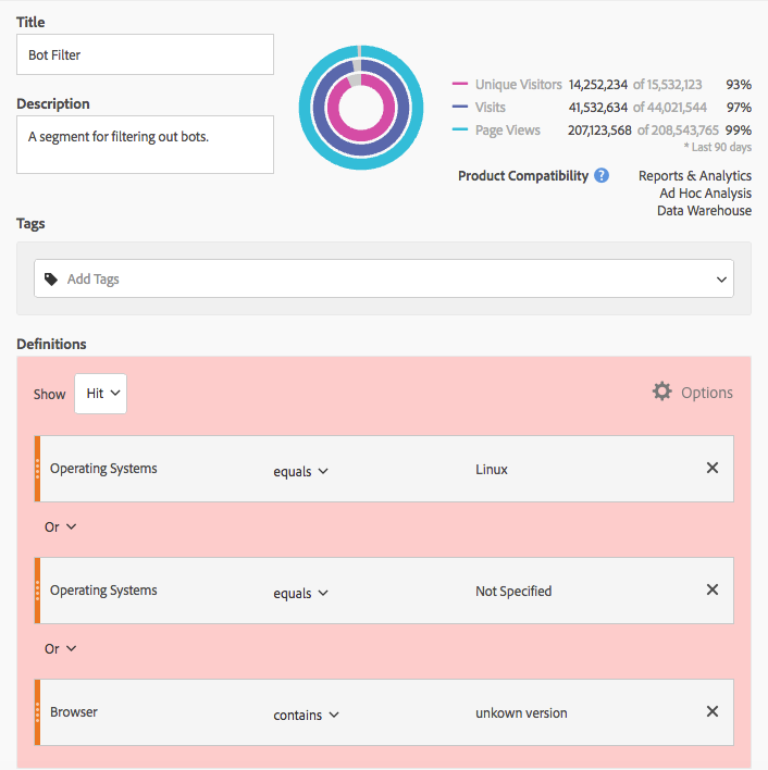
This method will miss a lot of the tricky bots, but should capture a a good number of bots without any extra work – Adobe Analytics already supports OS and Browser as segmentable dimensions.
- Using the approach outlined in my previous post, you can upload a Customer Attribute against all of the offending visitor IDs in your data. This requires you to upload a visitor classification file on a regular basis, but it is a lot more precise and the resulting Customer Attribute can be used as a segment definition as well.
In either case, once you have a bot filtering segment, I highly recommend creating a Virtual Report Suite based on your bot filtering segment to make sure you never see that corrupted data in your reporting again.
As a last thought, I also find it very interesting to report on the bot traffic itself in order to see the pages or times of day that bots hit the site:
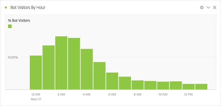
Notice how the bots really start hitting the site early in the morning – another calling card of bot traffic. I’ve also noticed that bots frequently go to product details pages more often because that’s where you find the prices – so be sure to apply a bot exclusion segment if you do a lot of analysis around product details pages!
To wrap up, bots are an ever growing problem and it’s important to understand how they impact your data. Protect yourself from bad analysis and bad conclusions by using some of the techniques I’ve shown you here. These techniques are certainly not the best or only way to filter bot traffic, but it’s certainly a lot better than nothing!